Benchmarking Coreset Algorithms

In this benchmark, we assess the performance of different coreset algorithms: KernelHerding, SteinThinning, RandomSample, RPCholesky, KernelThinning, and CompressPlusPlus. Each of these algorithms is evaluated across four different tests, providing a comparison of their performance and applicability to various datasets.

This benchmark only evaluates unsupervised coreset algorithms. Hence, the tasks involve selecting a representative subset of data points without any prior labels provided.

Test 1: Benchmarking Coreset Algorithms on the MNIST Dataset

The first test evaluates the performance of the coreset algorithms on the MNIST dataset using a simple neural network classifier. The process follows these steps:

1. Dataset: The MNIST dataset consists of 60,000 training images and 10,000 test images. Each image is a 28x28 pixel grey-scale image of a handwritten digit.

2. Model: A Multi-Layer Perceptron (MLP) neural network is used for classification. The model consists of a single hidden layer with 64 nodes. Images are flattened into vectors for input.

3. Dimensionality Reduction: To speed up computation and reduce dimensionality, a density preserving UMAP is applied to project the 28x28 images into 16 components before applying any coreset algorithm.

4. Coreset Generation: Coresets of various sizes are generated using the different coreset algorithms. For KernelHerding, SteinThinning, and KernelThinning, MapReduce is employed to handle large-scale data.

5. Training: The model is trained using the selected coresets, and accuracy is measured on the test set of 10,000 images.

6. Evaluation: Due to randomness in the coreset algorithms and training process, the experiment is repeated 4 times with different random seeds. The benchmark is run on an Amazon Web Services EC2 g4dn.12xlarge instance with 4 NVIDIA T4 Tensor Core GPUs, 48 vCPUs, and 192 GiB memory.

Impact of UMAP and MapReduce on Coreset Performance

In the benchmarking of coreset algorithms, only Random Sample can be run without MapReduce or UMAP without running into memory allocation errors. The other coreset algorithms require dimensionality reduction and distributed processing to handle large-scale data efficiently. As a result, the coreset algorithms were not applied directly to the raw MNIST images. While these preprocessing steps improved efficiency, they may have impacted the performance of the coreset methods. Specifically, MapReduce partitions the dataset into subsets and applies solvers to each partition, which can reduce accuracy compared to applying solvers directly to the full dataset. Additionally, batch normalisation and dropout were used during training to mitigate over-fitting. These regularisation techniques made the models more robust, which also means that accuracy did not heavily depend on the specific subset chosen. The benchmarking test showed that the accuracy remained similar regardless of the coreset method used, with only small differences, which could potentially be attributed to the use of these regularisation techniques.

Results: The accuracy of the MLP classifier when trained using the full MNIST dataset (60,000 training images) was 97.31%, serving as a baseline for evaluating the performance of the coreset algorithms.

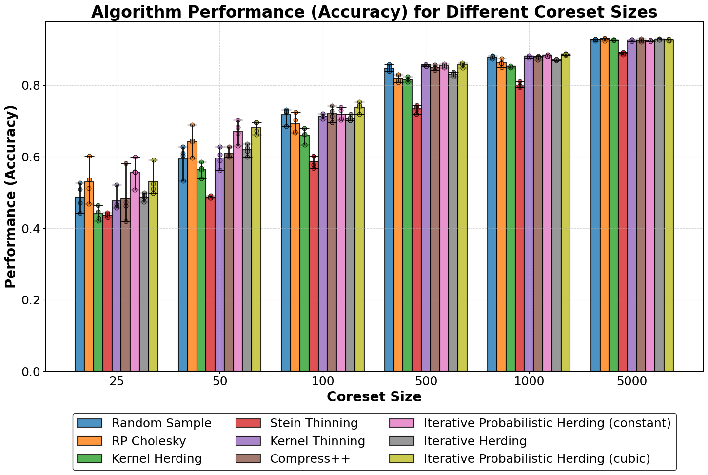
Figure 1: Accuracy of coreset algorithms on the MNIST dataset. Bar heights represent the average accuracy. Error bars represent the min-max range for accuracy for each coreset size across 5 runs.

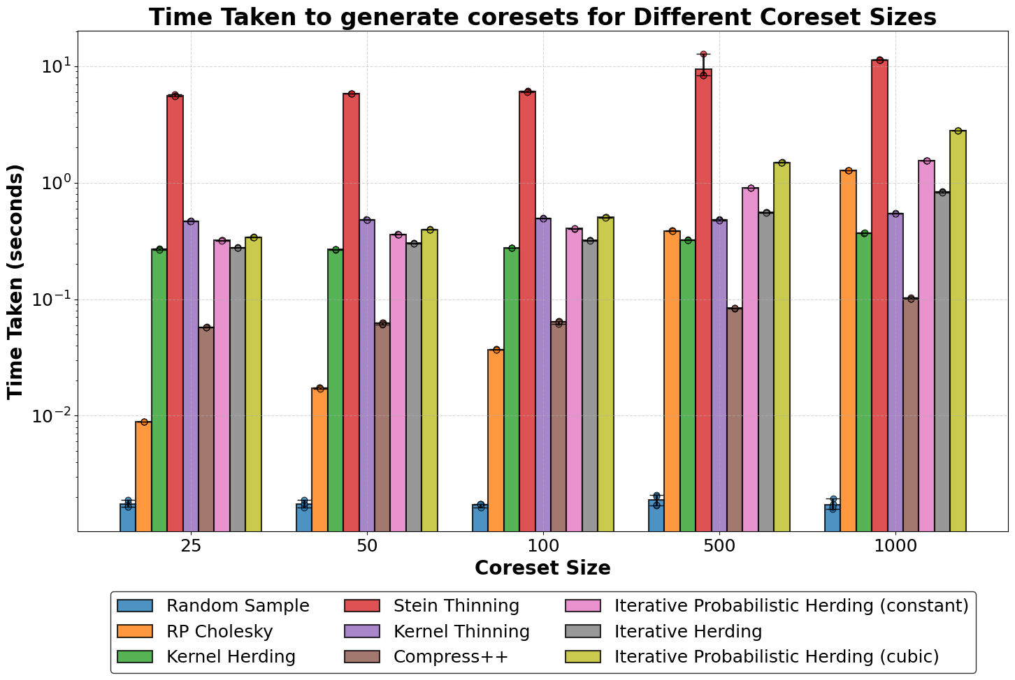
Figure 2: Time taken to generate coreset for each coreset algorithm. Bar heights represent the average time taken. Error bars represent the min-max range for each coreset size across 5 runs.

Test 2: Benchmarking Coreset Algorithms on a Synthetic Dataset

In this second test, we evaluate the performance of the coreset algorithms on a synthetic dataset. The dataset consists of 1,024 points in two-dimensional space, generated using sklearn.datasets.make_blobs(). The process follows these steps:

1. Dataset: A synthetic dataset of 1,024 points is generated to test the quality of coreset algorithms.

2. Coreset Generation: Coresets of different sizes (10, 50, 100, and 200 points) are generated using each coreset algorithm.

3. Evaluation Metrics: Two metrics evaluate the quality of the generated coresets: MMD and KSD.

4. Optimisation: We optimise the weights for coresets to minimise the MMD score and recompute both MMD and KSD metrics. These entire process is repeated 5 times with a different random seed each time and the metrics are averaged.

Results: The tables below show the performance metrics (Unweighted MMD, Unweighted KSD, Weighted MMD, Weighted KSD, and Time) for each coreset algorithm and each coreset size. For each metric and coreset size, the best performance score is highlighted in bold.

Coreset Size 25 (Original Sample Size 1,024)

Method	Unweighted_MMD	Unweighted_KSD	Weighted_MMD	Weighted_KSD	Time
KernelHerding	0.024273	0.086342	0.008471	0.074467	4.765064
RandomSample	0.111424	0.088141	0.011224	0.075859	3.372750
RPCholesky	0.140047	0.073147	0.003688	0.060939	4.026443
SteinThinning	0.144938	0.085247	0.063385	0.086622	5.611508
KernelThinning	0.014880	0.075884	0.005388	0.064494	25.014126
CompressPlusPlus	0.013212	0.084045	0.007081	0.081235	16.713568
ProbabilisticIterativeHerding	0.021128	0.089382	0.007852	0.080658	4.702327
IterativeHerding	0.007051	0.068399	0.005125	0.065863	3.825249
CubicProbIterativeHerding	0.004543	0.081827	0.003512	0.077990	4.375146

Coreset Size 50 (Original Sample Size 1,024)

Method	Unweighted_MMD	Unweighted_KSD	Weighted_MMD	Weighted_KSD	Time
KernelHerding	0.014011	0.057618	0.003191	0.052470	4.036918
RandomSample	0.104925	0.079876	0.004955	0.061597	3.279080
RPCholesky	0.146650	0.064917	0.001539	0.054541	3.720830
SteinThinning	0.086824	0.055094	0.013564	0.061475	4.627325
KernelThinning	0.006304	0.061570	0.002246	0.058513	14.038467
CompressPlusPlus	0.007616	0.063311	0.002819	0.056713	10.396490
ProbabilisticIterativeHerding	0.015108	0.068838	0.003151	0.063005	4.108718
IterativeHerding	0.003708	0.052616	0.002604	0.053199	3.577140
CubicProbIterativeHerding	0.001733	0.058076	0.001442	0.059921	4.120308

Coreset Size 100 (Original Sample Size 1,024)

Method	Unweighted_MMD	Unweighted_KSD	Weighted_MMD	Weighted_KSD	Time
KernelHerding	0.007909	0.046639	0.001859	0.051218	4.235977
RandomSample	0.055019	0.061831	0.001804	0.057107	3.158193
RPCholesky	0.097647	0.039633	0.001044	0.055332	3.850249
SteinThinning	0.093073	0.035877	0.006268	0.055652	4.740899
KernelThinning	0.002685	0.056104	0.001265	0.058189	9.000171
CompressPlusPlus	0.002936	0.055740	0.001226	0.055948	8.099011
ProbabilisticIterativeHerding	0.009710	0.062317	0.001838	0.059106	4.518486
IterativeHerding	0.002256	0.048805	0.001407	0.051166	4.135961
CubicProbIterativeHerding	0.000805	0.051934	0.000979	0.054329	4.499996

Coreset Size 200 (Original Sample Size 1,024)

Method	Unweighted_MMD	Unweighted_KSD	Weighted_MMD	Weighted_KSD	Time
KernelHerding	0.004259	0.047415	0.001173	0.054883	4.568870
RandomSample	0.041521	0.057967	0.000914	0.055495	3.401281
RPCholesky	0.056923	0.042466	0.000830	0.053957	4.136736
SteinThinning	0.104213	0.024422	0.003508	0.055823	5.040177
KernelThinning	0.001518	0.054005	0.000886	0.057455	6.787894
CompressPlusPlus	0.001410	0.053179	0.000755	0.054638	7.406790
ProbabilisticIterativeHerding	0.006358	0.058343	0.000873	0.057020	4.711837
IterativeHerding	0.001382	0.050098	0.000995	0.054194	4.150570
CubicProbIterativeHerding	0.000582	0.052761	0.000706	0.056212	4.702852

Visualisation: The results in this table can be visualised as follows:

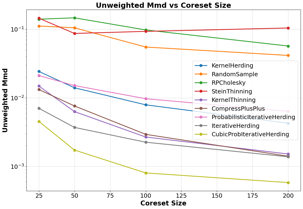
Figure 3: Unweighted MMD plotted against coreset size for each coreset method.

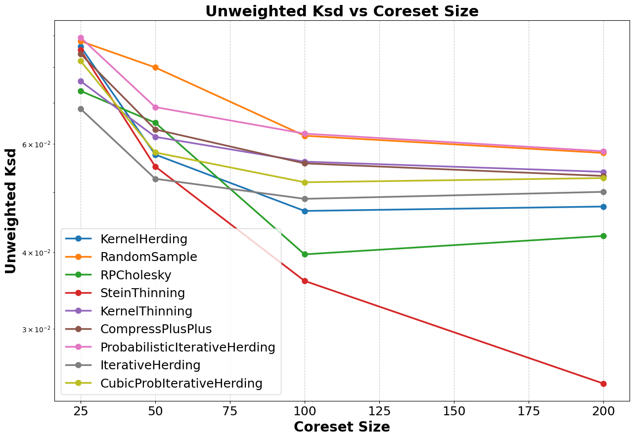
Figure 4: Unweighted KSD plotted against coreset size for each coreset method.

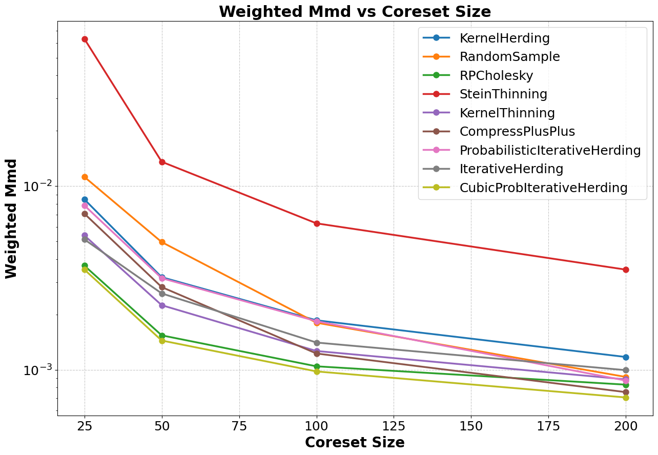
Figure 5: Weighted MMD plotted against coreset size for each coreset method.

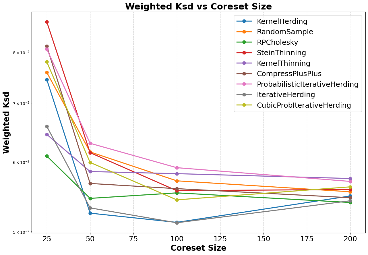
Figure 6: Weighted KSD plotted against coreset size for each coreset method.

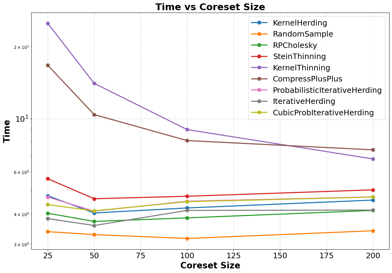
Figure 7: Time taken plotted against coreset size for each coreset method.

Test 3: Benchmarking Coreset Algorithms on Pixel Data from an Image

This test evaluates the performance of coreset algorithms on pixel data extracted from an input image. The process follows these steps:

1. Image Preprocessing: An image is loaded and converted to grey-scale. Pixel locations and values are extracted for use in the coreset algorithms.

2. Coreset Generation: Coresets (of size 20% of the original image) are generated using each coreset algorithm.

3. Visualisation: The original image is plotted alongside coresets generated by each algorithm. This visual comparison helps assess how well each algorithm represents the image.

Results: The following plot visualises the pixels chosen by each coreset algorithm.

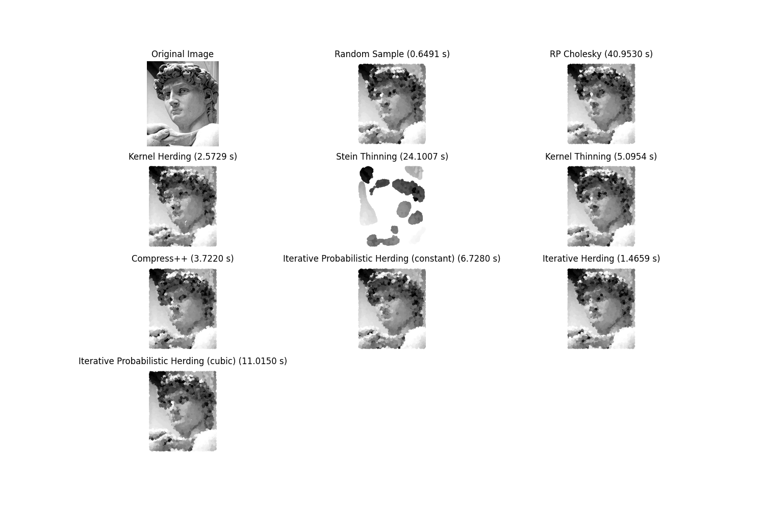
Figure 8: The original image and pixels selected by each coreset algorithm plotted side-by-side for visual comparison.

Test 4: Selecting Key Frames from Video Data

The fourth and final test evaluates the performance of coreset algorithms on data extracted from an input animated Video. This test involves the following steps:

1. Input Video: A video is loaded, and its frames are preprocessed.

2. Dimensionality Reduction: On each frame data, a density preserving UMAP is applied to reduce dimensionality of each frame to 25.

3. Coreset Generation: For each coreset algorithm, coresets are generated and selected frames are saved as new video.

Result: - Video files showing the selected frames for each coreset algorithm.

Video 1: Original video file.

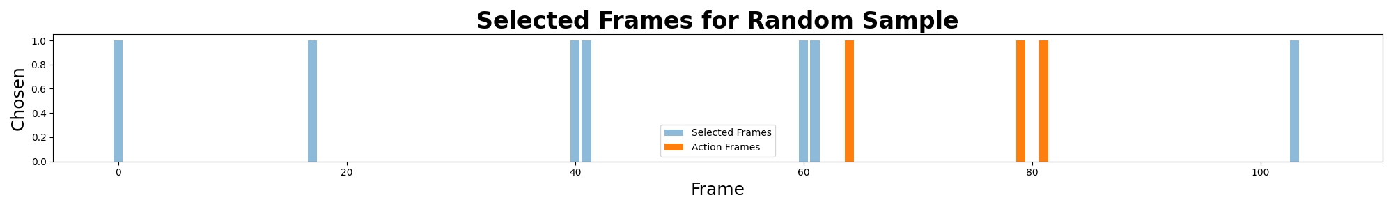
Video 2: Frames selected by Random Sample.

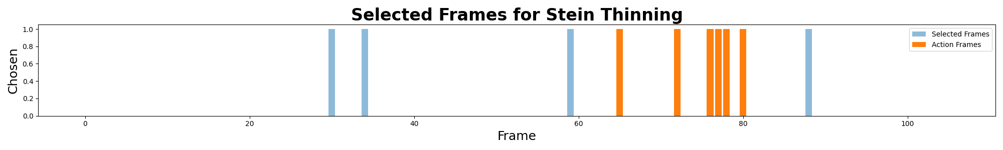
Video 3: Frames selected by Stein thinning.

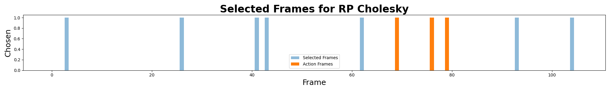
Video 4: Frames selected by RP Cholesky.

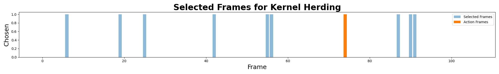
Video 5: Frames selected by Kernel Herding.

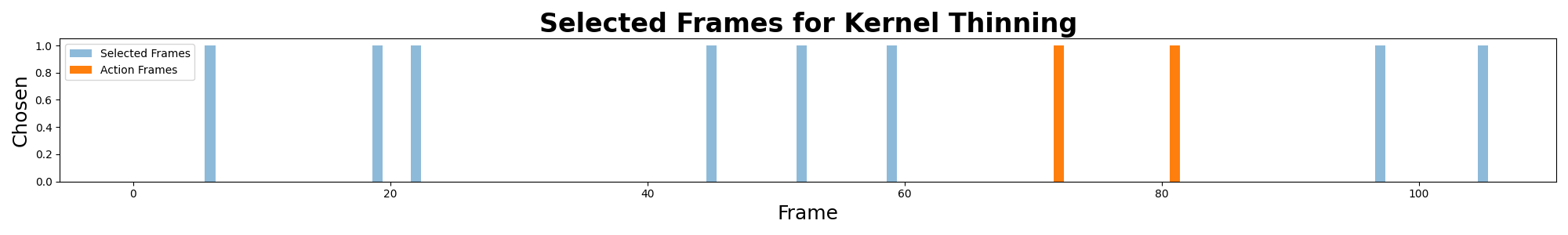
Video 6: Frames selected by Kernel Thinning.

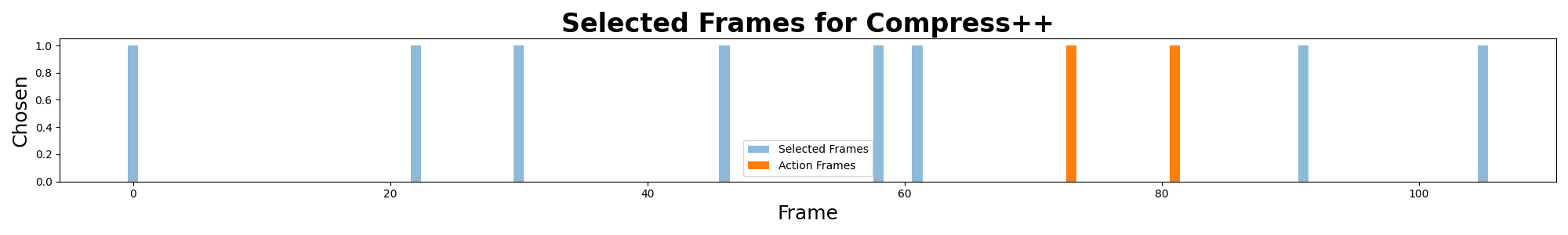
Video 7: Frames selected by Compress++.

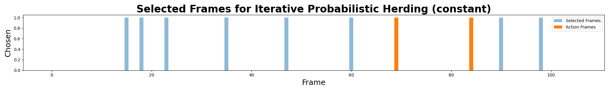
Video 8: Frames selected by Probabilistic Iterative Kernel Herding.

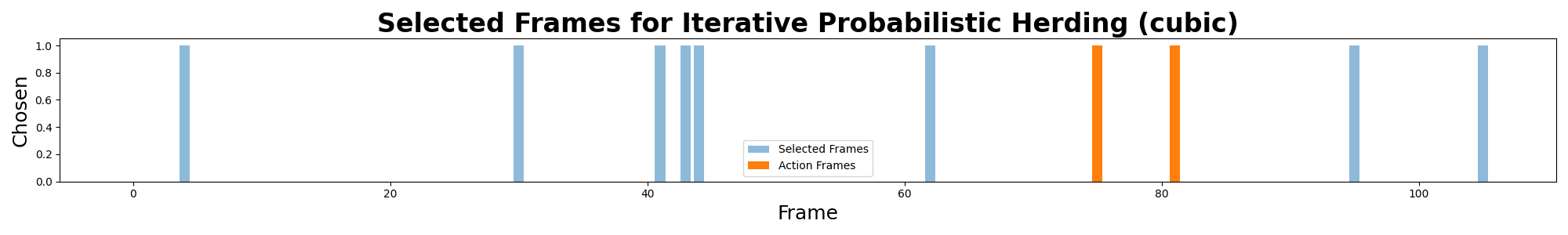
Video 8: Frames selected by Probabilistic Iterative Kernel Herding with a

decaying temperature parameter.

The following plots show the frames chosen by each coreset algorithm with action frames in orange.

Conclusion

This benchmark evaluated four coreset algorithms across various tasks, including image classification and frame selection. Iterative kernel herding and kernel thinning emerged as the top performers, offering strong and consistent results. For large-scale datasets, compress++ and map reduce provide efficient scalability.

Ultimately, this conclusion reflects one interpretation of the results, and readers are encouraged to analyse the benchmarks and derive their own insights based on the specific requirements of their tasks.