Analytical example with Stein Thinning

Step-by-step usage of the Stein Thinning algorithm ([liu2016kernelized], [benard2023kernel]) on a small example with 10 data points in 2 dimensions and selecting a 2 point coreset, i.e., \(N=10, m=2\).

For Stein Thinning, we need to provide a kernel and a score function, \(\nabla \log p(x)\), where \(p\) is the underlying distribution of the data. In practice, we can estimate this using methods such as kernel density estimation and sliced score matching [song2020ssm].

In this example we will use PCIMQ kernel with length_scale of \(\frac{1}{\sqrt{2}}\): for two points \(x, y \in X\), \(k(x, y) = \frac{1}{\sqrt{1+\| x - y \|^2}}\). We use the standard normal density \(p(x) \propto e^{-\|x\|^2/2}\), so the score function is \(s_p(x) = -x\).

The first step of the algorithm is to convert the given kernel into a Stein kernel using the given score function. The Stein kernel between points \(x\) and \(y\) is given as:

\[\begin{split}k_p(x,y) &= \langle \nabla_\mathbf{x}, \nabla_{\mathbf{y}} k(\mathbf{x}, \mathbf{y}) \rangle + \langle s_p(\mathbf{x}), \nabla_{\mathbf{y}} k(\mathbf{x}, \mathbf{y}) \rangle + \langle s_p(\mathbf{y}), \nabla_\mathbf{x} k(\mathbf{x}, \mathbf{y}) \rangle + \langle s_p(\mathbf{x}), s_p(\mathbf{y}) \rangle k(\mathbf{x}, \mathbf{y}) \\ & = -3\|x-y\|^2(1 + \|x-y\|^2)^{-5/2} + (d - \|x-y\|^2)(1 + \|x-y\|^2) ^{-3/2} + (x\cdot y)(1 + \|x-y\|^2)^{-1/2}\end{split}\]

Now the algorithm proceeds iteratively, selecting the next point greedily by minimising the regularised KSD metric:

\[x_{t} = \arg\min_{x} \left( k_p(x, x) + \Delta^+ \log p(x) - \lambda t \log p(x) + 2\sum_{j=1}^{t-1} k_p(x, x_j) \right)\]

Note that the Laplacian regularisation term (\(\Delta^+ \log p(x)\)) vanishes for the given score function. Hence, using \(k_p(x,y)\) and \(p(x)\) given above, we have:

\[\begin{split}k_p(x, x) &= d + \|x\|^2 \\ \Delta^+ \log p(x) &= 0 \\ - \lambda t \log p(x) &= \frac{\lambda t}{2} \|x\|^2 \\\end{split}\]

We can now simplify the metric at iteration \(t\) in this example:

\[d + \|x\|^2(1 + \lambda t/2) + 2\sum_{j=1}^{t-1} k_p(x_{j}, x)\]

For now let’s suppose no regularisation (\(\lambda = 0\)) and selecting a unique point at each iteration. We now select points iteratively by minimizing the metric at each step.

Let’s suppose we have the following data:

\[\begin{split}X = \begin{pmatrix} -0.1 & -0.1 \\ -0.3 & -0.2 \\ -0.2 & 0.6 \\ 0.8 & 0.2 \\ -0.0 & 0.3 \\ 0.9 & -0.7 \\ 0.2 & -0.1 \\ 0.7 & -1.0 \\ -0.4 & -0.4 \\ 0.0 & -0.3 \end{pmatrix}\end{split}\]

First iteration (t=1):

In the first iteration there are no previously selected points, hence we simply compute \(k_p(x, x) = d + \| x \|^2\) for each point:

\[\begin{split}\text{KSD}(X) = \begin{pmatrix} 2.020 \\ 2.130 \\ 2.400 \\ 2.680 \\ 2.090 \\ 3.300 \\ 2.050 \\ 3.490 \\ 2.320 \\ 2.090 \end{pmatrix}\end{split}\]

We select point at index 0 (assuming 0-indexing), \((-0.1, -0.1)\), as it has the minimum score of 2.020.

Second iteration (t=2):

We now have to additionally compute \(k_p(x, X[0])\) for each point since \(X[0]\) was selected in the first iteration:

\[\begin{split}\text{KSD}(X) = \begin{pmatrix} 6.060 \\ 5.587 \\ 2.879 \\ 2.290 \\ 4.238 \\ 2.673 \\ 4.952 \\ 2.889 \\ 4.593 \\ 5.508 \end{pmatrix}\end{split}\]

We now select the point at index 3, \((0.8, 0.2)\), with the corresponding score of 2.290.

Third iteration (t=3):

We now compute \(k_p(x, X[3])\) for each point and update the scores:

\[\begin{split}\text{KSD}(X) = \begin{pmatrix} 5.670 \\ 4.618 \\ 2.339 \\ 7.650 \\ 4.490 \\ 3.393 \\ 5.894 \\ 2.710 \\ 3.377 \\ 5.187 \end{pmatrix}\end{split}\]

We select the point at index 2, \((-0.2, 0.6)\), with the corresponding score of 2.339.

Note that selecting a particular point changes the metric significantly at each iteration, emphasising that the algorithm attempts to move away from the already selected points and explore the rest of the space.

The final selected points are \(\{0, 3, 2\}\) with corresponding data points:

\[\begin{split}X_{\text{coreset}} = \begin{pmatrix} -0.1 & -0.1 \\ 0.8 & 0.2 \\ -0.2 & 0.6 \end{pmatrix}\end{split}\]

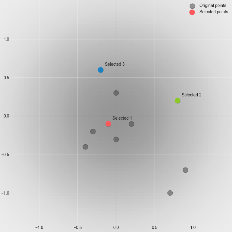
The underlying probability density (standard normal) corresponding to our score function is shown in the background. The algorithm will have a tendency to sample points according to the density.

Non-unique Coreset Points

It is possible for Stein Thinning to select the same point repeatedly. For instance, in the example above, if we proceed with the procedure for 10 iterations we get the following sequence of selected indices: \(0, 3, 2, 7, 8, 2, 5, 8, 3, 2\).

We can set unique=True in the SteinThinning solver to prevent this from happening . In this case, the score of a selected point is always set to \(\infty\) after the iteration.

Regularisation

When regularisation Stein Thinning is used (regularise=True), extra regularisation terms are added to the KSD metric. In particular, in our example, the additional term is \(-\lambda t \log p(x)\) where \(p\) is the density, \(t\) is the current iteration and \(\lambda\) is the regularisation parameter.

Note that the SteinThinning solver uses a Gaussian KDE estimate of \(p\) since it might not be possible to deduce it directly from the score function.

If we use this estimate, set \(\lambda=1\) and repeat the procedure above, we get the following sequence of selected indices: \(0, 2, 5, 8, 6, 3, 1, 4, 7, 9\).