Benchmarking Coreset Algorithms

In this benchmark, we assess the performance of four different coreset algorithms: KernelHerding, SteinThinning, RandomSample, RPCholesky and KernelThinning. Each of these algorithms is evaluated across four different tests, providing a comparison of their performance and applicability to various datasets.

Test 1: Benchmarking Coreset Algorithms on the MNIST Dataset

The first test evaluates the performance of the coreset algorithms on the MNIST dataset using a simple neural network classifier. The process follows these steps:

1. Dataset: The MNIST dataset consists of 60,000 training images and 10,000 test images. Each image is a 28x28 pixel grey-scale image of a handwritten digit.

2. Model: A Multi-Layer Perceptron (MLP) neural network is used for classification. The model consists of a single hidden layer with 64 nodes. Images are flattened into vectors for input.

3. Dimensionality Reduction: To speed up computation and reduce dimensionality, a density preserving UMAP is applied to project the 28x28 images into 16 components before applying any coreset algorithm.

4. Coreset Generation: Coresets of various sizes are generated using the different coreset algorithms. For KernelHerding and SteinThinning, MapReduce is employed to handle large-scale data.

5. Training: The model is trained using the selected coresets, and accuracy is measured on the test set of 10,000 images.

6. Evaluation: Due to randomness in the coreset algorithms and training process, the experiment is repeated 4 times with different random seeds. The benchmark is run on an Amazon Web Services EC2 g4dn.12xlarge instance with 4 NVIDIA T4 Tensor Core GPUs, 48 vCPUs, and 192 GiB memory.

Results: The accuracy of the MLP classifier when trained using the full MNIST dataset (60,000 training images) was 97.31%, serving as a baseline for evaluating the performance of the coreset algorithms.

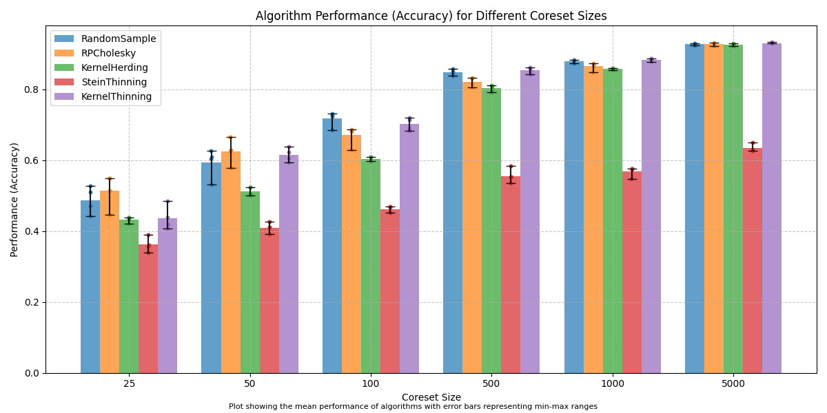
Figure 1: Accuracy of coreset algorithms on the MNIST dataset. Bar heights represent the average accuracy. Error bars represent the min-max range for accuracy for each coreset size across 5 runs.

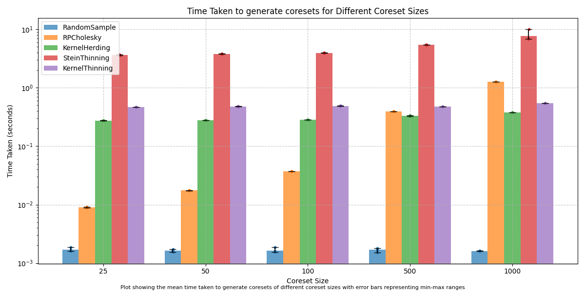
Figure 2: Time taken to generate coreset for each coreset algorithm. Bar heights represent the average time taken. Error bars represent the min-max range for each coreset size across 5 runs.

Test 2: Benchmarking Coreset Algorithms on a Synthetic Dataset

In this second test, we evaluate the performance of the coreset algorithms on a synthetic dataset. The dataset consists of 1,000 points in two-dimensional space, generated using sklearn.datasets.make_blobs(). The process follows these steps:

1. Dataset: A synthetic dataset of 1,000 points is generated to test the quality of coreset algorithms.

2. Coreset Generation: Coresets of different sizes (10, 50, 100, and 200 points) are generated using each coreset algorithm.

3. Evaluation Metrics: Two metrics evaluate the quality of the generated coresets: MMD and KSD.

4. Optimisation: We optimise the weights for coresets to minimise the MMD score and recompute both MMD and KSD metrics. These entire process is repeated 5 times with a different random seed each time and the metrics are averaged.

Results: The tables below show the performance metrics (Unweighted MMD, Unweighted KSD, Weighted MMD, Weighted KSD, and Time) for each coreset algorithm and each coreset size. For each metric and coreset size, the best performance score is highlighted in bold.

Coreset Size 25 (Original Sample Size 1,000)

Method	Unweighted_MMD	Unweighted_KSD	Weighted_MMD	Weighted_KSD	Time
KernelHerding	0.026319	0.071420	0.008461	0.072526	1.836664
RandomSample	0.105940	0.081013	0.038174	0.077431	1.281091
RPCholesky	0.121869	0.059722	0.003283	0.072288	1.576841
SteinThinning	0.161923	0.077394	0.030987	0.074365	1.821020
KernelThinning	0.014111	0.072134	0.006634	0.072531	9.144707

Coreset Size 50 (Original Sample Size 1,000)

Method	Unweighted_MMD	Unweighted_KSD	Weighted_MMD	Weighted_KSD	Time
KernelHerding	0.012574	0.072600	0.003843	0.072351	1.863356
RandomSample	0.083379	0.079031	0.008653	0.072867	1.329118
RPCholesky	0.154799	0.056437	0.001347	0.072359	1.564009
SteinThinning	0.122605	0.079683	0.012048	0.072424	1.849748
KernelThinning	0.005397	0.072051	0.002191	0.072453	5.524234

Coreset Size 100 (Original Sample Size 1,000)

Method	Unweighted_MMD	Unweighted_KSD	Weighted_MMD	Weighted_KSD	Time
KernelHerding	0.007651	0.071999	0.001814	0.072364	2.185324
RandomSample	0.052402	0.077454	0.001630	0.072480	1.359826
RPCholesky	0.087236	0.063822	0.000910	0.072433	1.721290
SteinThinning	0.128295	0.082733	0.006041	0.072182	1.893099
KernelThinning	0.002591	0.072293	0.001207	0.072394	3.519274

Coreset Size 200 (Original Sample Size 1,000)

Method	Unweighted_MMD	Unweighted_KSD	Weighted_MMD	Weighted_KSD	Time
KernelHerding	0.004310	0.072341	0.000777	0.072422	1.837929
RandomSample	0.036624	0.072870	0.000584	0.072441	1.367439
RPCholesky	0.041140	0.068655	0.000751	0.072430	2.106838
SteinThinning	0.148525	0.087512	0.003799	0.072164	1.910560
KernelThinning	0.001330	0.072348	0.001014	0.072428	2.565189

Visualisation: The results in this table can be visualised as follows:

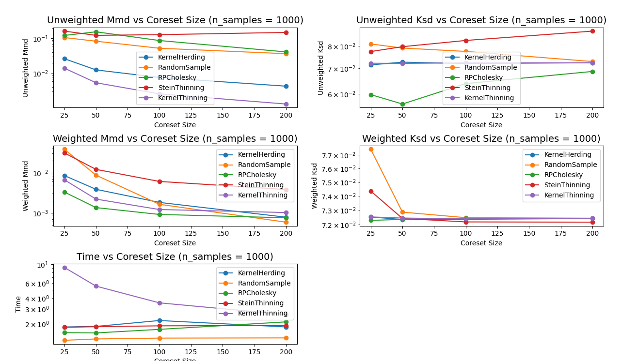
Figure 3: Line graphs depicting the average performance metrics across 5 runs of each coreset algorithm on a synthetic dataset.

Test 3: Benchmarking Coreset Algorithms on Pixel Data from an Image

This test evaluates the performance of coreset algorithms on pixel data extracted from an input image. The process follows these steps:

1. Image Preprocessing: An image is loaded and converted to grey-scale. Pixel locations and values are extracted for use in the coreset algorithms.

2. Coreset Generation: Coresets (of size 20% of the original image) are generated using each coreset algorithm.

3. Visualisation: The original image is plotted alongside coresets generated by each algorithm. This visual comparison helps assess how well each algorithm represents the image.

Results: The following plot visualises the pixels chosen by each coreset algorithm.

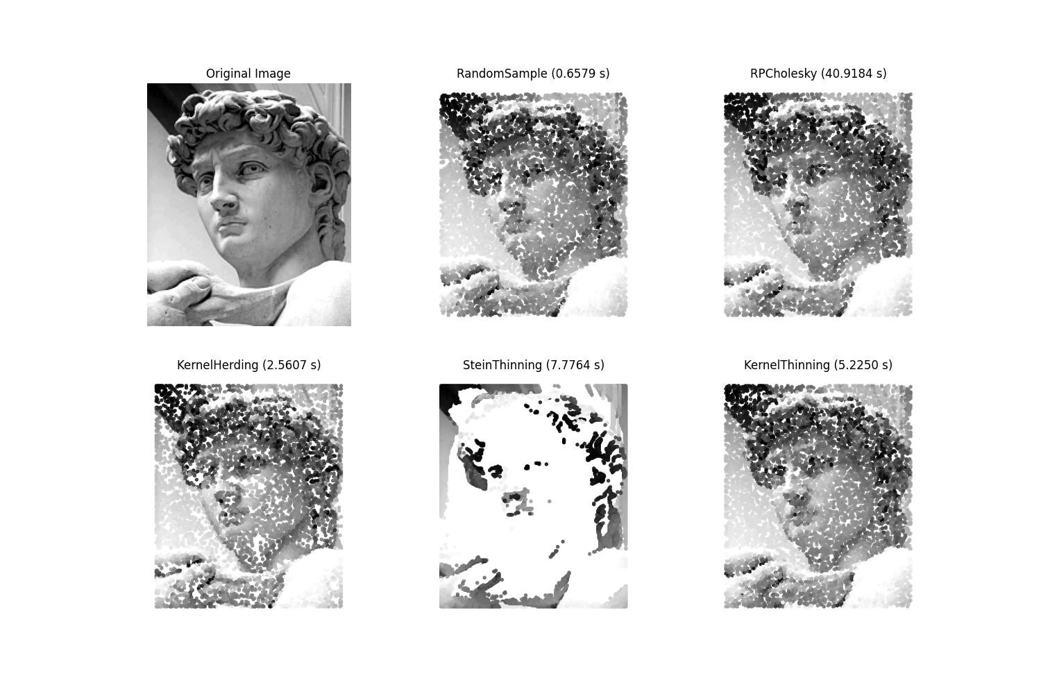
Figure 4: The original image and pixels selected by each coreset algorithm plotted side-by-side for visual comparison.

Test 4: Benchmarking Coreset Algorithms on Frame Data from a GIF

The fourth and final test evaluates the performance of coreset algorithms on data extracted from an input GIF. This test involves the following steps:

1. Input GIF: A GIF is loaded, and its frames are preprocessed.

2. Dimensionality Reduction: On each frame data, a density preserving UMAP is applied to reduce dimensionality of each frame to 25.

3. Coreset Generation: Coresets are generated using each coreset algorithm, and selected frames are saved as new GIFs.

Result: - GIF files showing the selected frames for each coreset algorithm.

Gif 1: Original gif file.

Gif 2: Frames selected by Random Sample.

Gif 3: Frames selected by Stein thinning.

Gif 4: Frames selected by RP Cholesky.

Gif 5: Frames selected by kernel herding.

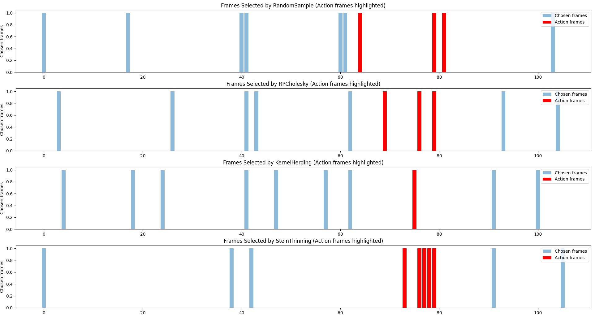
Figure 5:Frames chosen by each each coreset algorithm with action frames (the frames in which pounce action takes place) highlighted in red.

Conclusion

In this benchmark, we evaluated four coreset algorithms across various datasets and tasks, including image classification, synthetic datasets, and pixel/frame data processing. Based on the results, kernel thinning emerges as the preferred choice for most tasks due to its consistent performance. For larger datasets, combining kernel herding with distributed frameworks like map reduce is recommended to ensure scalability and efficiency.

For specialised tasks, such as frame selection from GIFs (Test 4), Stein thinning demonstrated superior performance and may be the optimal choice.

Ultimately, this conclusion reflects one interpretation of the results, and readers are encouraged to analyse the benchmarks and derive their own insights based on the specific requirements of their tasks.